On a remote sensor the binding constraint is not compute, it is bandwidth.
Sending raw signal is what drains the budget, so the question is how much of the
signal can be reconstructed after squeezing it through a model small enough to
run on the microcontroller itself.
Constraints
Microcontroller-class hardware. Kilobytes of RAM, no room for a general-purpose runtime, and a model that has to fit in flash alongside the application.
Reconstruction has to stay faithful. Compression that loses the signal defeats the point of collecting it.
The budget is power, not time. Encoding has to cost less energy than transmitting the bytes it saves, or the whole exercise is negative.
The target is an ESP32 class device, which is what fixes the third constraint in
place: the encoder has to share flash with the application, so the model budget
is whatever is left over rather than whatever the model wants.
How it's built
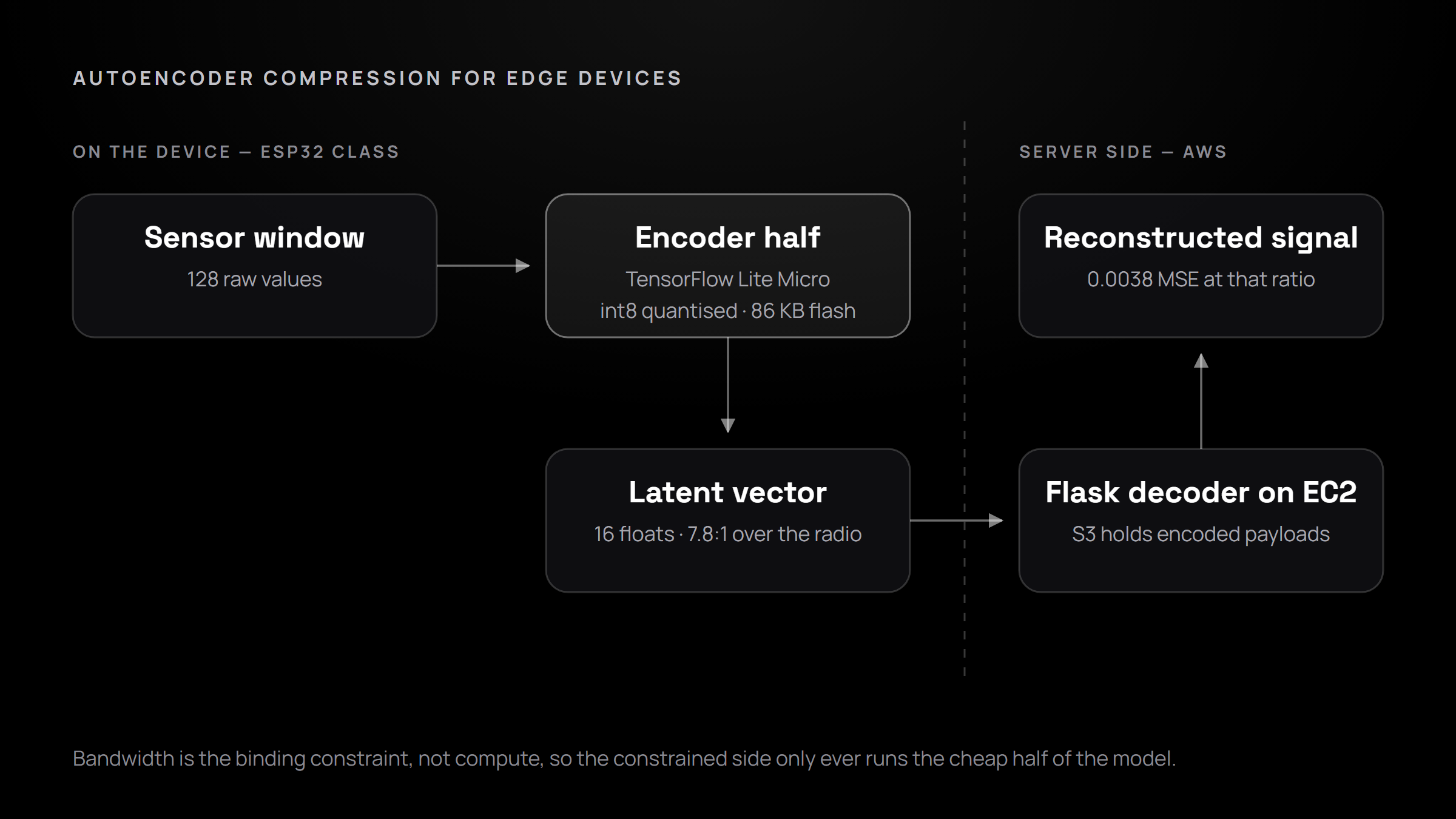
An autoencoder is trained offline on representative sensor data. The encoder
half is converted to TensorFlow Lite Micro and flashed to the device, where it
turns each reading window into a small latent vector that goes over the radio.
The decoder half sits behind a Flask API on AWS EC2 and reconstructs the
original signal server-side, with S3 holding encoded payloads.The asymmetry is the entire design. The constrained side only ever runs the
cheap half.
Scroll to see the whole diagramThe split that is the whole design: the device runs only the encoder, and the half that costs memory runs where memory is free.Sizing the latent vector, and getting it wrong first. The first latent size I
tried was too aggressive. It fit comfortably and reconstructed badly, in a way
that was easy to miss because average error looked acceptable while the sharp
transitions in the signal, the part actually worth transmitting, were being
smoothed away. Mean error is the wrong lens for this: it rewards a model that
reproduces the boring middle of the distribution. Widening the latent vector
fixed the reconstruction and moved the problem to memory, which is where the
quantisation work came in. The final encoder is integer-quantised and sized to
leave headroom in flash for the application rather than consuming everything
available.Measured:
Compression ratio: 7.8:1 versus raw readings
Reconstruction error: 0.0038 MSE at that ratio
Latent vector: 16 floats, down from 128 raw values
Encoder footprint on-device: 86 KB
Trade-offs I made
Lossy learned compression over lossless encoding. The autoencoder reaches
7.8:1 by accepting reconstruction error a lossless codec never introduces. The
cost is that the decoded signal is an approximation and its error tolerance has
to be stated, not assumed. The benefit is a compression ratio lossless approaches
cannot reach on this signal.Splitting the model across the boundary. The encoder runs on-device through
TensorFlow Lite Micro; the decoder runs server-side on EC2. The cost is that the
two halves must stay version-compatible across deployments. The benefit is that
the device carries only the half that must be small.An autoencoder rather than a general-purpose compressor. Generic compression
is domain-blind. An autoencoder trained on this sensor's actual distribution
learns what is signal and what is noise for this data specifically, and reaches a
much smaller representation at equal fidelity. The cost is that the model is
useless on a different sensor, which is an acceptable trade for a fixed
deployment.Quantised encoder over a smaller float model. TF Lite Micro wants integer
arithmetic, and quantising a well-sized model beat shrinking a float one at the
same footprint.
What I'd do differently
I tuned latent size against reconstruction error alone. The metric that actually
decides whether this project pays for itself is energy per encode measured
against energy saved per transmission, and I never measured it. A model that
compresses 7.8:1 while costing more power to run than the radio saves is a net
loss, and I cannot currently prove it is not. That measurement comes first next
time.I would also have chosen the error metric before the latent size rather than
after. Mean squared error was the default, and it is the metric that hid the
first failure: it rewarded a model that smoothed away exactly the sharp
transitions the sensor exists to capture. I found that by looking at
reconstructions, not by measuring. Picking a metric that weights transitions
properly would have made the first attempt fail loudly instead of quietly, which
is the whole point of having a metric.
I’m open to full-time backend, platform and data engineering roles, and happy to walk through any decision on this page in more detail than it deserves.